Factor correlations with 90-day forward returns. Power Law Deviation shows the strongest relationship.
I set out to determine which factors most reliably predict Bitcoin's forward returns, and specifically how to handle situations where different signals conflict.
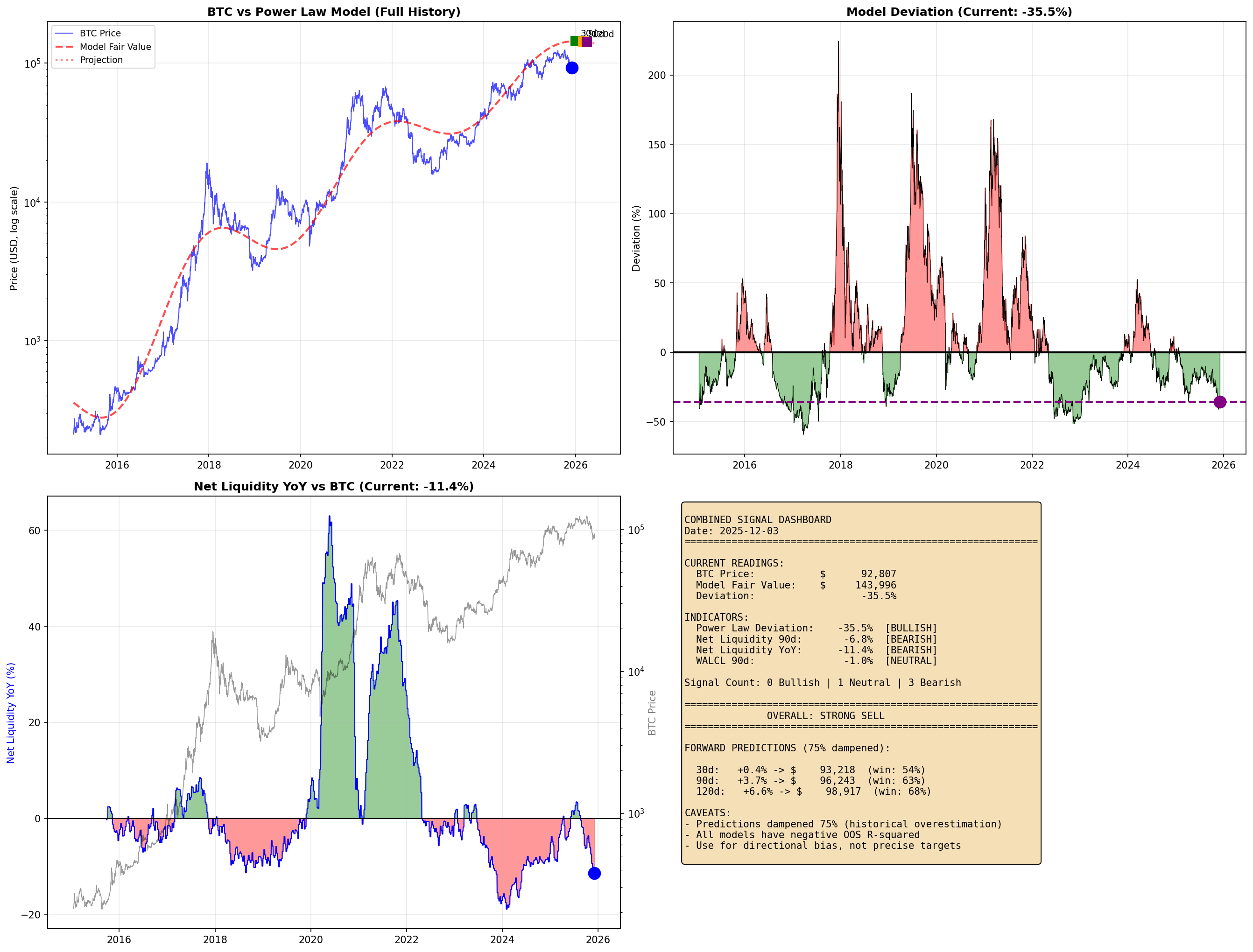
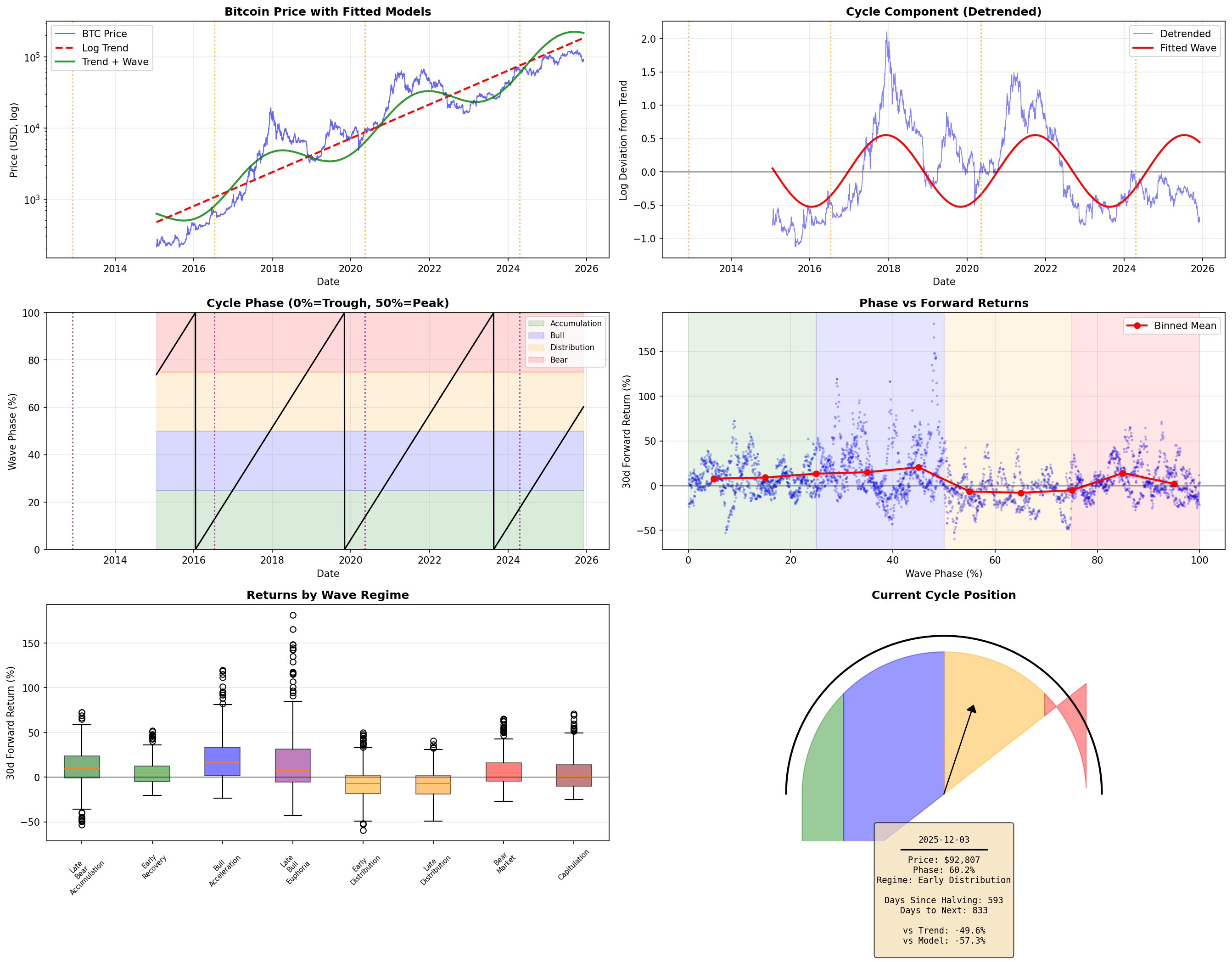
I'm currently observing conflicting signals:
This raised a practical question: when signals disagree, which should take precedence?
I selected three factors, each representing a distinct hypothesis about what drives Bitcoin returns.
Bitcoin follows a long-term logarithmic growth trajectory, and deviations from this trend tend to mean-revert.
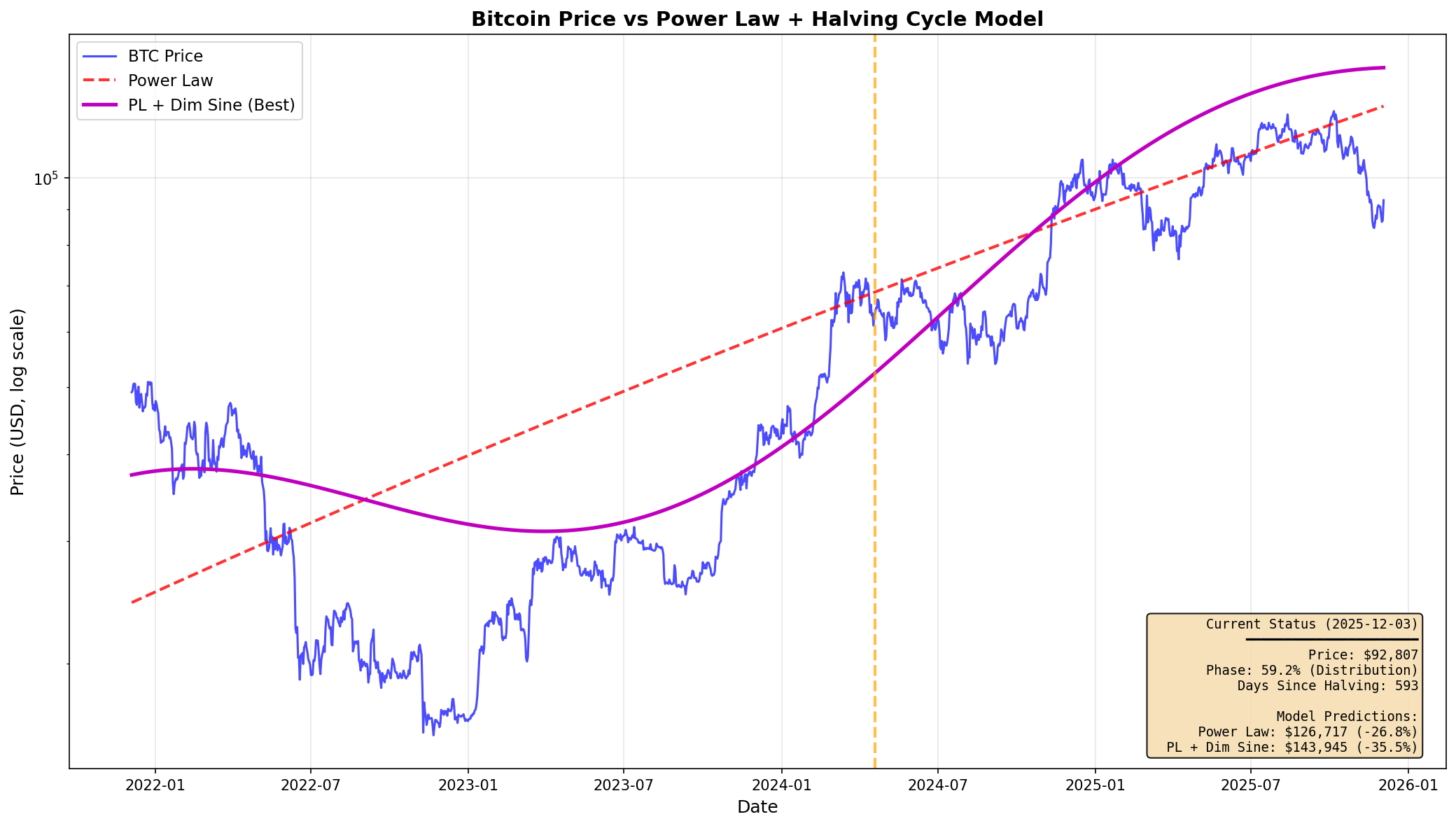
Several researchers (notably Giovanni Santostasi) have observed that Bitcoin's price, when plotted on log-log axes against time, follows a remarkably linear path. This suggests a power law relationship: price grows as a function of time raised to some exponent.
The intuition is that Bitcoin's value derives from network effects (Metcalfe's Law), and network growth follows predictable adoption curves. If true, significant deviations from the trend represent mispricing—overvaluation eventually corrects down, undervaluation corrects up.
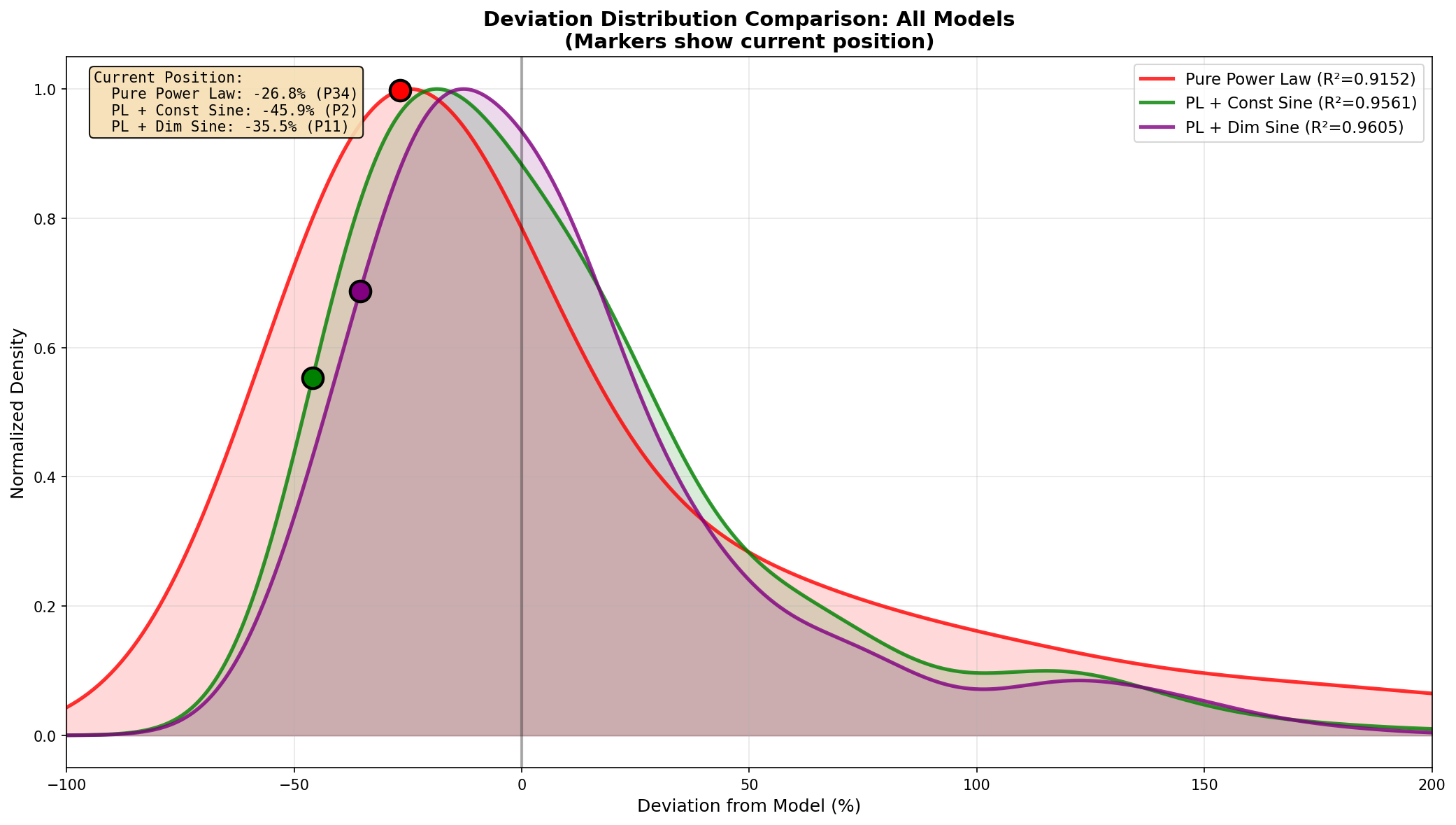
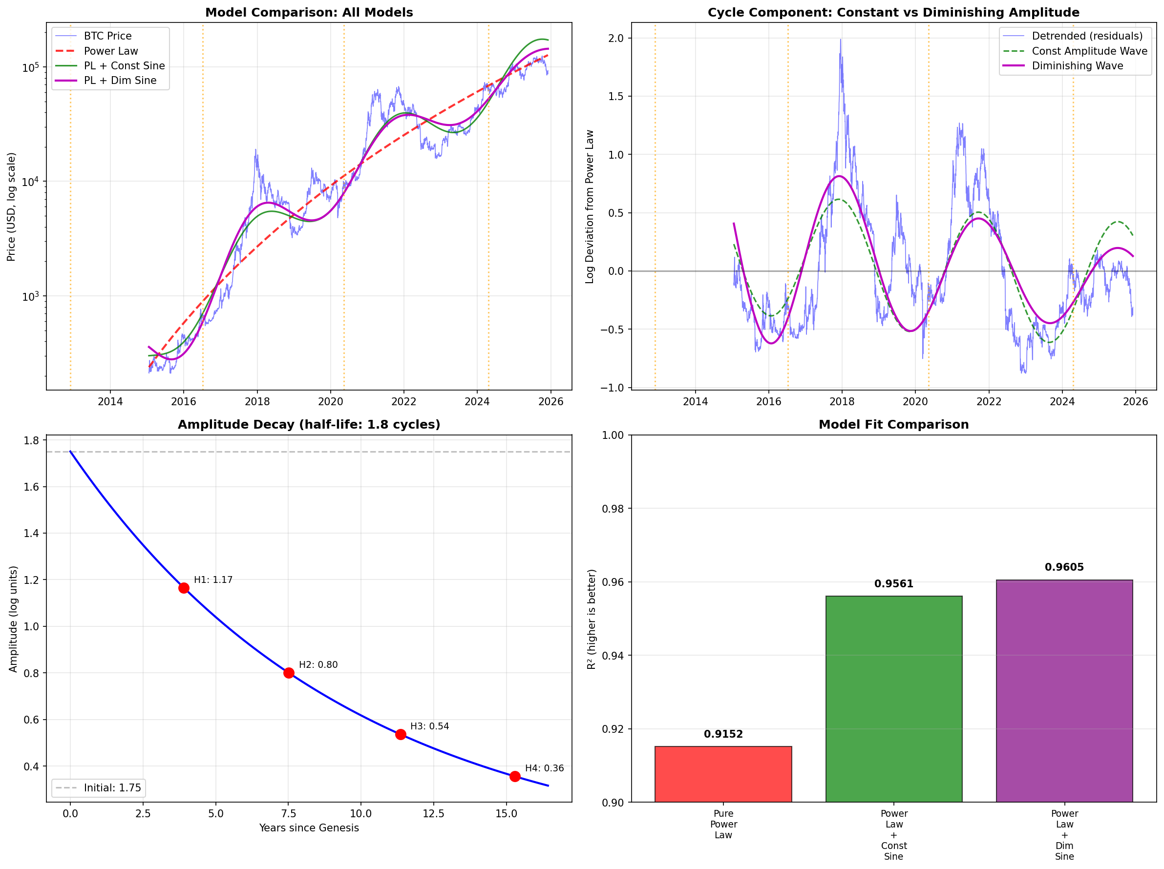
I fitted a power law model with a damped sinusoidal component to capture cyclical behavior. The model achieves R² = 0.96, indicating strong fit to historical data.
Bitcoin's fixed supply schedule creates predictable market cycles tied to halving events.
Every ~4 years, the Bitcoin block reward halves, cutting the rate of new supply in half. This is a fundamental, programmatic feature of Bitcoin that cannot be changed.
The halving creates a supply shock: miners receive fewer BTC for the same work, reducing sell pressure. Historically, this has preceded bull markets. The cycle appears to follow a pattern:
Unlike most market cycles, the halving is scheduled years in advance. This makes it a unique, exogenous timing signal.
Bitcoin, as a risk asset, responds to broader liquidity conditions in the financial system.
Since 2020, Bitcoin has increasingly correlated with traditional risk assets. The proposed mechanism:
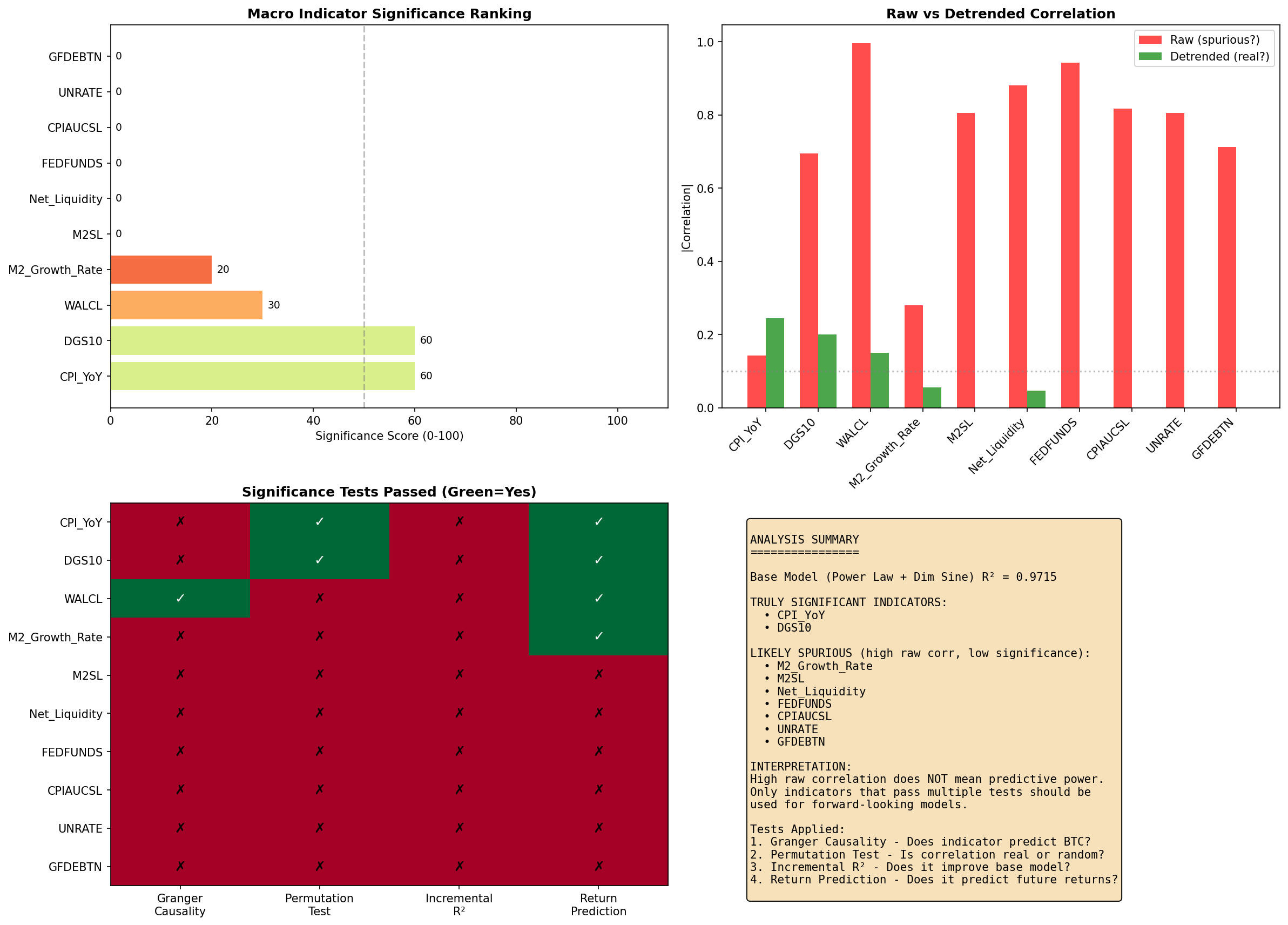
I examined several macro indicators:
The question was whether these macro factors add predictive value beyond Bitcoin-specific factors.
I first measured how each factor correlates with 90-day forward returns across the full dataset.
| Rank | Factor | Correlation | p-value |
|---|---|---|---|
| 1 | Power Law Deviation | -0.449 | 1.50e-191 |
| 2 | Halving Phase | -0.289 | 7.91e-76 |
| 3 | 10Y Yield 90d Change | -0.276 | 3.34e-67 |
| 4 | Days from Halving | -0.274 | 5.91e-68 |
| 5 | M2 YoY | +0.186 | 1.77e-29 |
| 6 | WALCL YoY | +0.184 | 4.94e-29 |
Observation: Power Law Deviation shows the strongest single-factor correlation. Based on this alone, I would have concluded it should be the primary signal.
I then examined return distributions within each factor's subgroups.
| Quintile | Description | Mean 90d Return | Win Rate |
|---|---|---|---|
| Q1 | Very Undervalued | +31.1% | 82.1% |
| Q2 | Undervalued | +28.7% | 77.3% |
| Q3 | Fair Value | +16.7% | 69.1% |
| Q4 | Overvalued | +4.8% | 54.6% |
| Q5 | Very Overvalued | -10.9% | 31.7% |
Q1 vs Q5 spread: +42.0% (t=26.71, p<0.001)
| Phase | Days Post-Halving | Mean 90d Return | Win Rate |
|---|---|---|---|
| Pre-Halving | -547 to 0 | +17.1% | 70.2% |
| Post-Halving Bull | 0 to 547 | +27.5% | 77.0% |
| Distribution | 547 to 1095 | -26.3% | 10.6% |
Bull vs Distribution spread: +53.7% (t=30.97, p<0.001)
Observation: Both factors show statistically significant return differentials. The question remained: what happens when they conflict?
This was the critical test. I isolated observations where Power Law indicated "undervalued" (deviation < -20%) and examined how returns varied by halving phase.
| Scenario | N | Mean 90d Return | Win Rate |
|---|---|---|---|
| Undervalued + Pre-Halving | 279 | +26.4% | 93.5% |
| Undervalued + Bull Phase | 368 | +50.3% | 100% |
| Undervalued + Distribution | 130 | -13.3% | 6.9% |
Key finding: The same "undervalued" reading produces a 63.6 percentage point difference in average returns depending on phase. During Distribution, the undervaluation signal not only fails to predict positive returns—it coincides with negative returns.
I ran the reverse test to check whether undervaluation provides any benefit during Distribution:
| During Distribution | N | Mean 90d Return | Win Rate |
|---|---|---|---|
| Undervalued | 130 | -13.3% | 6.9% |
| Fair Value | 287 | -28.1% | 9.4% |
| Overvalued | 236 | -31.8% | 14.0% |
Undervaluation is the least negative outcome, but still produces losses. The phase effect dominates.
| Test | Statistic | p-value |
|---|---|---|
| T-test: Undervalued+Bull vs Undervalued+Distribution | t = 18.05 | < 0.001 |
| ANOVA: Phase effect within Q1 | F = 142.3 | < 0.001 |
| Permutation test (10,000 iterations) | 0 exceeded observed | < 0.0001 |
The interaction effect is statistically robust.
The initial finding that Power Law has higher correlation (-0.449 vs -0.289) appeared to contradict the interaction analysis. I resolved this as follows:
The -0.449 correlation is computed across all 3,971 observations. This average blends:
The aggregate correlation masks regime-dependent performance. Power Law's predictive power is conditional on phase.
This leads to a hierarchical interpretation:
Halving Phase functions as a regime filter that determines whether valuation-based signals are actionable.
| Factor | Value | Standalone Interpretation |
|---|---|---|
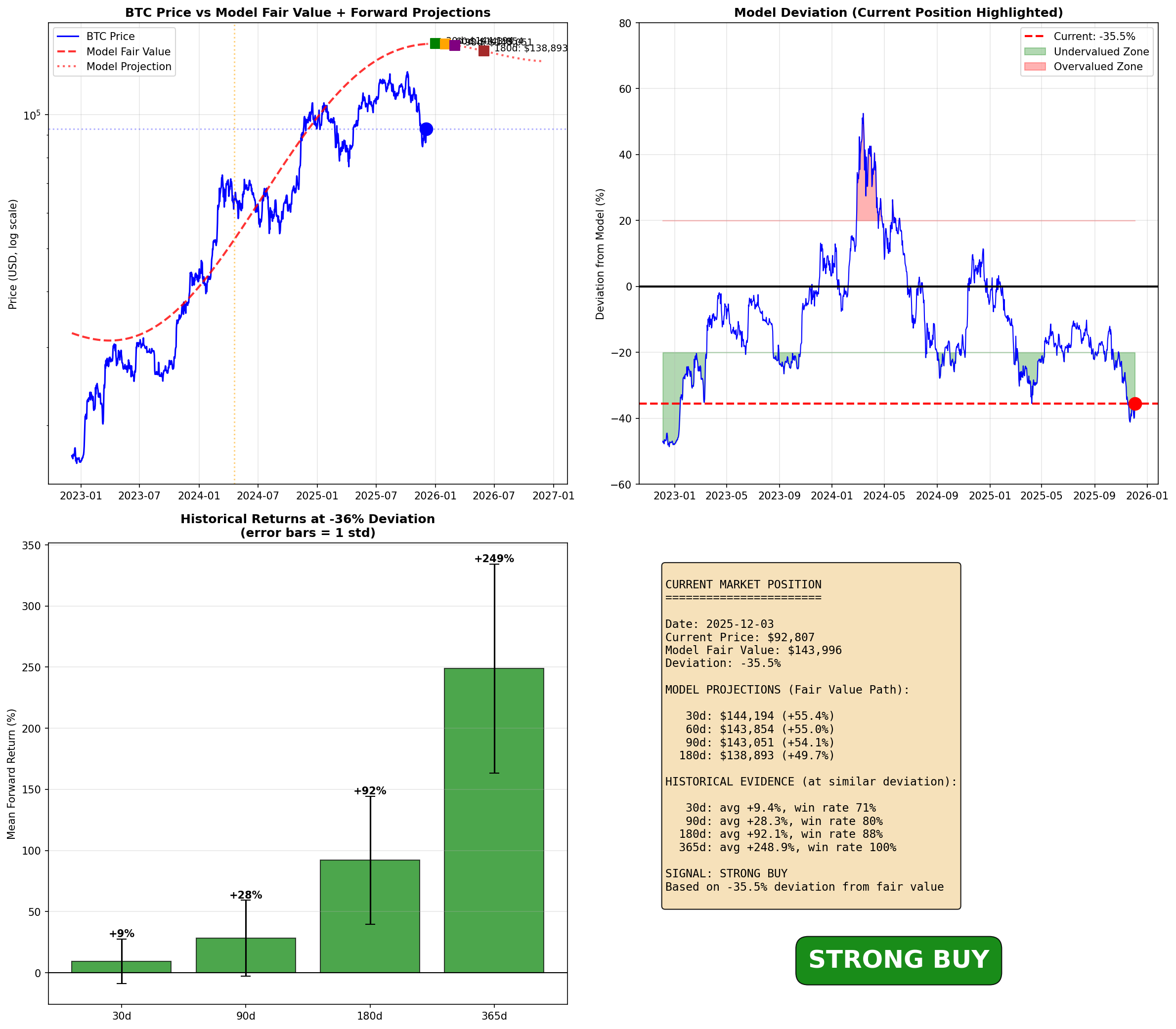
| Power Law Deviation | -35.5% | Undervalued |
| Halving Phase | Day 593 | Distribution |
| Net Liquidity 90d | -6.8% | Contracting |
I filtered for observations matching the current setup: undervalued + Distribution phase.
| Metric | Value |
|---|---|
| Sample size | 159 |
| Mean 90d return | -16.6% |
| Median 90d return | -14.9% |
| Win rate | 5.7% |
| 5th percentile | -38.2% |
| 95th percentile | +4.2% |
| Percentile | 90d Return |
|---|---|
| 5th | -38.2% |
| 25th | -17.4% |
| 50th | -14.9% |
| 75th | -7.9% |
| 95th | +4.2% |
Even at the 90th percentile, the outcome was approximately breakeven.
Based on the evidence, the current outlook is negative despite the undervaluation reading. The Power Law signal is not reliable during Distribution phase. Historical precedent for this configuration shows a 5.7% win rate with mean returns of -16.6%.
log(P) = a + b*log(t) + A*e^(-decay*t/T)*sin(2π*t/T + φ)

Parameters:
- t = days since genesis (Jan 3, 2009)
- T = halving cycle length (1,387 days)
- Fitted values: a=-38.19, b=5.71, A=1.75, φ=-0.71, decay=0.40
- R² = 0.9605Halving Dates:
- 2012-11-28
- 2016-07-09
- 2020-05-11
- 2024-04-19
Phase Boundaries (days from halving):
- Pre-Halving: -547 to 0
- Post-Halving Bull: 0 to 547
- Distribution: 547 to 1095| PL Dev | Phase | Days | M2 | WALCL | |
|---|---|---|---|---|---|
| PL Dev | 1.00 | 0.42 | 0.38 | -0.21 | -0.18 |
| Phase | 0.42 | 1.00 | 0.89 | -0.15 | -0.12 |
| Days | 0.38 | 0.89 | 1.00 | -0.11 | -0.09 |
| M2 YoY | -0.21 | -0.15 | -0.11 | 1.00 | 0.87 |
| WALCL | -0.18 | -0.12 | -0.09 | 0.87 | 1.00 |